Different or Equivalent?

When we show that the results of our study are "statistically significant" we feel that the study was worth the effort, that we have met our objectives. This is because the current meaning of the word "significant" implies that something is important or consequential but, unfortunately, that was not its intended meaning. (See John Cook's blog "The Endeavor" for a nice post on the Origin of “statistically significant”).

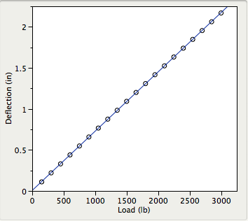
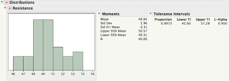
Let's say we need to to make a claim about the average DC resistance of a certain type of cable we manufacture. We set up the null hypothesis as μ=50 Ohm vs. the alternative hypothesis μ≠50 Ohm, and measure the resistance of 40 such cables. If the one-sample t-test, based on the sample of 40 cables, is statistically significant we can claim that the average DC resistance is different from 50 Ohm. Our claim does not imply that this difference is of any practical importance, this depends on the size of the difference, just that the average DC resistance is not 50 Ohm. A test of significance is a test of difference. This is the operational definition given to the term "statistical significance" by Sir Ronald Fisher in his 1925 book Statistical Methods for Research Workers: “Critical tests of this kind may be called tests of significance, and when such tests are available we may discover whether a second sample is or is not significantly different from the first" (emphasis mine).

What if we do not reject the null hypothesis μ=50 Ohm? Although tests of significance are set up to demonstrate difference not equality, we sometimes take this lack of evidence as evidence that the average DC resistance is in fact 50 Ohm. This is because in practice we encounter situations where we need to demonstrate to a customer, or government agency, that the average DC resistance is "close" to 50 Ohm. In the context of significance testing what we need to do is to swap the null and alternative hypothesis and test for equivalence within a given bound; i.e., test μ≠50 Ohm vs. |μ-50 Ohm|< δ, where δ is a small number. In the next post Brenda discusses how a test of equivalence is a great way of combining statistical with practical significance.

Looks Like a Straight Line to Me

The graph below shows 40 Deflection (in) vs Load (lb) measurements (open circles), and its least squares fit (blue line). The straight line seems to fit the behavior of the data well, with an, almost perfect, RSquare equal to 99.9989%.

(Data available from National Institute of Standards and Technology (NIST))

Do you think the straight line is a good fit for Deflection as a function of Load?

The RSquare tells us that 99.9989% of the variation observed in the Deflection data is explained by the linear relationship, so based on this criteria this seems like a pretty good fit. However, a single measure, like RSquare, does not give us the complete picture of how well a model approximates the data. In my previous post I wrote that a model is just a recipe for transforming data into noise. How do we check that what is left behind is noise? Residual plots provide a way to evaluate the residuals (=Data - Model), or what is left after the model is fit.

There are many types of residual plots that are used to assess the quality of the fit. A plot of the (studentized) residuals vs. predicted Deflection, for example, clearly shows that the linear model did not leave behind noise, but it failed to account for a quadratic term.

But based on the RSquare the fit is almost perfect, you protest. A statistical analysis does not exist in isolation but depends on the context of the data, the uncertainties we need to answer, and the assumptions we make. This data was collected to develop a calibration curve for load cells for which a highly accurate model is desired. The quadratic model explains 99.9999900179% of the variation in the Deflection data.

The quadratic model increases the precision of the coefficients, and prediction of future values, by reducing the Root Mean Square Error (RMSE) from 0.002171 to 0.0002052. A plot of the (studentized) residuals vs. Load now shows that what is left behind now is just noise.

For a complete analysis of the Deflection data see Chapter 7 of our book Analyzing and Interpreting Continuous Data Using JMP.

3 Is The Magic Number

I'm sure that I am about to date myself here, but who remembers Schoolhouse Rock in the 1970's? One of my favorite songs was 'Three is a Magic Number', which Jack Johnson later adapted in his song '3R's' from the Curious George soundtrack. I wonder if Bob Dorough was thinking about statistics when he came up with that song. Certainly, 3 is a number that seems to have some significance in a couple of important areas related to engineering. For instance, in Statistical Process Control (SPC), upper and lower control limits are typically 3 standard deviations on either side of the center line. And when fitness-for-use information is unknown, some may set specification limits for key attributes of a product, component, or raw material, based upon process capability, using the formula mean ±3×(standard deviation).

For a normal distribution we expect 99.73% of the population to be between ±3x(standard deviation). In fact, for many distributions most of the population is contained between ±3x(standard deviation), hence the "magic" of the number 3. For control charts, using 3 as the multiplier, was well justified by Walter Shewhart because it provides a good balance between chasing down false alarms and missing signals due to assignable causes. However, when it comes to setting specification limits, the value 3 in the formula mean ±3×(standard deviation) may not contain 99.73% of the population unless the sample size is very large.

Using "3" to set specification limits assumes that we know, without error, the true population mean and standard deviation. In practice, we almost never know the true population parameters and we must estimate them from a random and, usually small, representative sample. Luckily for us, there is a statistical interval called a tolerance interval that takes into account the uncertainty of the estimates of the mean and standard deviation and the sample size, and is well suited for setting specification limits. The interval has the form mean ±k×(standard deviation), with k being a function of the confidence, the sample size, and the proportion of the population we want the interval to contain (99.73% for an equivalent ±3×(standard deviation) interval).

Consider an example using 40 resistance measurements taken from 40 cables. The JMP output for a tolerance interval that contains 99.73% of the population, indicates that with 95% confidence, we expect 99.73% of the resistance measurements to be between 42.60 Ohm and 57.28 Ohm. These values should be used to set our lower and upper specification limits, instead of mean ±3×(standard deviation).

To learn more about tolerance intervals see Statistical Intervals.